Markov chain Monte Carlo (MCMC) methods provide powerful and widely applicable algorithms for simulating from probability distributions, including complex and high-dimensional distributions.

It is combined with two parts, Markov Chain and Monte Carlo.

1. Monte Carlo

Monte Carlo is a method that generate random numbers to deal with some problems. One classic method to generate random number is called Middle-Square Method

For example, we can use Monte Carlo Method to estimate the value of \(\pi\).

2. Markov Chain

A. Markov Property

In Stochastic Process, if one specific time is \(x_n\), then the probability of \(x_{n+1}\) is called Markov Property. In probability theory and statistics, the term Markov property refers to the memoryless property of a stochastic process.

In Mathematical Formula, it can be written as:

So, if one process has Stochastic Process, it can also be called Markov Process.

B. The Stationary Distribution

For example, you have a Transition Rate Matrix, and you write it as \(Q\).

For example, we have our \(Q\) matrix as: \(\begin{equation*} \begin{bmatrix} 0.9 & 0.075 & 0.025 \\ 0.15 & 0.8 & 0.05 \\ 0.25 & 0.25 & 0.5 \end{bmatrix} \end{equation*}\)

Suppose we have \(3\) points, then \(Q_{11}\) means the probability from point A to itself is \(0.9\).

Suppose our orignal state is \(s_0=[0,1,0]\), then the probability of next statement will be \(s_1=s_0 Q = [0.15,0.8,0.05]\). So, \(s_2=s_1 Q=s_0 Q^2\).

Stationary Distribution means we will get one Stationary statement such that \(sQ=s\), it can also be written as \(s(Q-I)=0\), then we call this \(s\) as Stationary Distribution.

From above example, our final Stationary Distribution \(s = [0.625, 0.315, 0.0625]\). Whatever your orignal state is, your final Stationary Distribution will be the same.

The stationary state distribution is important because it lets you define the probability for every state of a system at a random time.

3. MCMC

After introduced Monte Carlo and Markov Chain, then let’s get the definition of Markov Chain Monte Carlo. For example, if we already know the probability density function of one distribution (like \(\beta\) Distribution), how can we get the sample from this distribution?

MCMC provides us an algorithm that generate random sample from distribution. First, we need to know the following equations.

• Bayes Theorem: \(p(H\|D)=\frac{p(D\|H)p(H)}{p(D)}\)

• Prior Probability: \(p(H)\)

• Posterior Probability: \(p(H\|D)\)

• Likelihood: \(p(D\|H)\)

• Evidence: \(p(D)\)

If it’s continuous, then \(p(D)=\int_{H}p(H,D)dH\), if it’s discrete, then \(p(D)=\sum_{H}p(H,D)\). \(f(D)\) can be seen as a constant.

Metropolis-Hasting Algorithm

If \(s=(s_1,s_2,...,s_M)\) is the Stationary Distribution we want. Then, we need to construct a Markov Chain that contains this stationary distribution. So, this Markov Chain has \(M\) states, and \(p_{ij}\) in transition rate matrix \(P\) means the probability from \(i\) to \(j\).

Then, we need to do:

1. Choose a random orignal state \(i\).

2. Randomly choose a Proposal State, \(j\). It’s depend on the \(i\)-th row in matrix \(P\).

3. Calculate the acceptance probability, the formula is: \(\alpha_{ij}=min(\frac{s_j p_{ji}}{s_i p_{ij}}, 1)\)

4. Randomly choose a number between \(0\) and \(1\), if it’s bigger than \(0.5\), then accept. Otherwise, reject.

5. Repeat the process.

Finally, we can get our Stationary Distribution \(s\), then the Stationary Distribution is our target sample that we want to generate.

For example

If our target distribution is \(\beta\) distribution, and suppose in our matrix \(P\), \(p_{ij}=p_{ji}\) then:

MCMC in Python

Sampling from \(\beta\) distribution.

import random
# Lets define our Beta Function to generate s for any particular state. 
# We don't care for the normalizing constant here.

def beta_s(w,a,b): # beta distribution pdf
    return w**(a-1)*(1-w)**(b-1)

# This Function returns True if the coin with probability P of heads comes heads when flipped.
def random_coin(p):
    unif = random.uniform(0,1)
    if unif>=p:
        return False
    else:
        return True

# This Function runs the MCMC chain for Beta Distribution.
def beta_mcmc(N_hops,a,b):
    states = []
    cur = random.uniform(0,1)
    for i in range(0,N_hops):
        states.append(cur)
        next = random.uniform(0,1)
        ap = min(beta_s(next,a,b)/beta_s(cur,a,b),1) # Calculate the acceptance probability
        if random_coin(ap):
            cur = next
    return states[-1000:] # Returns the last 1000 states of the chain

import numpy as np
from matplotlib import pylab as plt
import scipy.special as ss

# Actual Beta PDF.
def beta(a, b, i):
    e1 = ss.gamma(a + b)
    e2 = ss.gamma(a)
    e3 = ss.gamma(b)
    return (e1/(e2*e3)) * (i ** (a - 1)) * ((1 - i) ** (b - 1))

# Create a function to plot Actual Beta PDF with the Beta Sampled from MCMC Chain.
def plot_beta(a, b):
    Ly = []
    Lx = []
    i_list = np.mgrid[0:1:100j]
    for i in i_list:
        Lx.append(i)
        Ly.append(beta(a, b, i))
    pl.plot(Lx, Ly, label="Real Distribution: a="+str(a)+", b="+str(b))
    plt.hist(beta_mcmc(100000,a,b),density=True,bins =25, 
            histtype='step',label="Simulated_MCMC: a="+str(a)+", b="+str(b))
    pl.legend()
    pl.show()
    
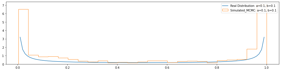
plot_beta(0.1, 0.1)
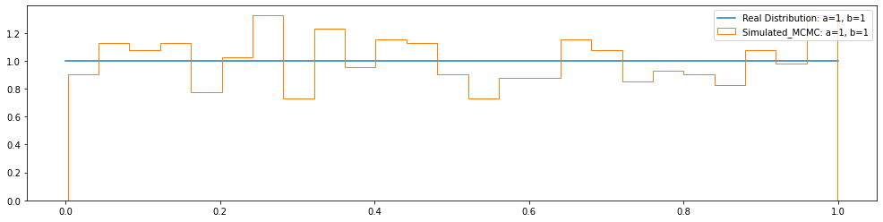
plot_beta(1, 1)
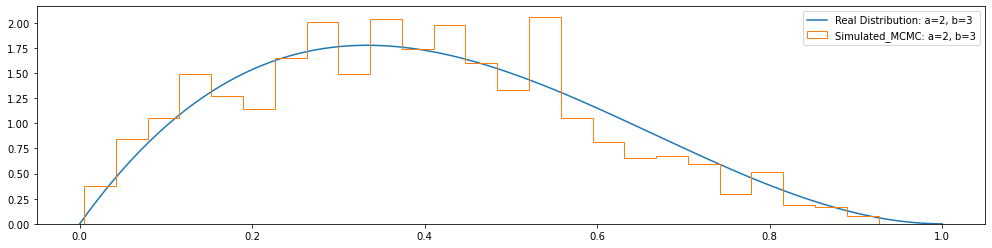
plot_beta(2, 3)